3.3 数据转换 (Data Transformation)
数据转换,简而言之,就是对原有数据的展示形式做一些改动,因而把最有意义的数值以易读的形式展示出来,或是为绘图做准备。
3.3.1 取子集(抓取行,列)
本小节介绍了如何使用dplyr 包提供的select(), filter(), slice取子集方法
更详细的解释请看第3.4.1.2节。
这一小节我们使用名为iris的数据。它是一个dataframe,所以首先把它转换成tibble.
iris <- as_tibble(datasets::iris)
iris
#> # A tibble: 150 x 5
#> Sepal.Length Sepal.Width Petal.Length Petal.Width Species
#> <dbl> <dbl> <dbl> <dbl> <fct>
#> 1 5.1 3.5 1.4 0.2 setosa
#> 2 4.9 3 1.4 0.2 setosa
#> 3 4.7 3.2 1.3 0.2 setosa
#> 4 4.6 3.1 1.5 0.2 setosa
#> 5 5 3.6 1.4 0.2 setosa
#> 6 5.4 3.9 1.7 0.4 setosa
#> 7 4.6 3.4 1.4 0.3 setosa
#> 8 5 3.4 1.5 0.2 setosa
#> 9 4.4 2.9 1.4 0.2 setosa
#> 10 4.9 3.1 1.5 0.1 setosa
#> # … with 140 more rows3.3.1.1 抓取单列
抓取单列很简单,也很常用(比如我们只想从一个大的tibble中抓两个变量研究它们之间的关系)。 有两个符号可以用于抓取列,$(仅用于变量名称)与[[]](变量名称或索引)。还是以mpg为例,假设我们要抓取第2列 (Sepal.Width):
# 通过变量名称抓取 -----------------------
iris[["Sepal.Width"]]
#或
iris$Sepal.Width #

# 通过索引抓取 ------------------------
iris[[2]]
以上三种方法都应得到同样的结果(是一个vector):
#>  [1] 3.5 3.0 3.2 3.1 3.6 3.9 3.4 3.4 2.9 3.1 3.7 3.4 3.0 3.0 4.0 4.4 3.9
#> [18] 3.5 3.8 3.8一般,在RStudio中使用$符号最方便,因为打出“$”之后会自动提示变量名。
一般我们抓取单列是为了在tibble中新建一个与那一列相关的变量,或是建一个新tibble,或是做统计学分析。以上三种情况(是绝大多数的情况)用vector进行操作很方便。
使用单方括号[进行取子集得到的结果是一个tibble(试试iris[2])这个特性在第3.4.1.2节中有解释。
3.3.1.2 使用select()函数,抓取多列并返回一个tibble
有时候,一个tibble中含有很多冗余信息,我们可能想把感兴趣的几个变量抓出来做一个新tibble. 这时select()函数最为方便。可以用变量名称或者索引来抓取;可以在前面加上负号表示“除这个变量以外”。比如:
iris_1 <- select(iris, 1:2, 5)
# 等同于
iris_1 <- select(iris, -(3:4))
# 等同于
iris_1 <- select(iris, -Petal.Length, -Petal.Width)

head(iris_1, 3) # 节省空间,1至3行。
#> # A tibble: 3 x 3
#> Sepal.Length Sepal.Width Species
#> <dbl> <dbl> <fct>
#> 1 5.1 3.5 setosa
#> 2 4.9 3 setosa
#> 3 4.7 3.2 setosa使用“正”的变量名称进行抓取,可以额外地按照你指定的顺序重排(抓取的是同样的数据,但是Species被放在第一列):
iris_1 <- select(iris, Species, Sepal.Length, Sepal.Width)
head(iris_1, 3)
#> # A tibble: 3 x 3
#> Species Sepal.Length Sepal.Width
#> <fct> <dbl> <dbl>
#> 1 setosa 5.1 3.5
#> 2 setosa 4.9 3
#> 3 setosa 4.7 3.2你还可以在变量名之间使用冒号:
iris_1 <- select(iris, Species, Sepal.Length:Petal.Length)
head(iris_1, 3)
#> # A tibble: 3 x 4
#> Species Sepal.Length Sepal.Width Petal.Length
#> <fct> <dbl> <dbl> <dbl>
#> 1 setosa 5.1 3.5 1.4
#> 2 setosa 4.9 3 1.4
#> 3 setosa 4.7 3.2 1.3你还可以通过变量名的命名规则来抓取:
iris_2 <- select(iris, Species, ends_with("Length"))
head(iris_2, 3)
#> # A tibble: 3 x 3
#> Species Sepal.Length Petal.Length
#> <fct> <dbl> <dbl>
#> 1 setosa 5.1 1.4
#> 2 setosa 4.9 1.4
#> 3 setosa 4.7 1.3iris_3 <- select(iris, Species, starts_with("Sepal"))
head(iris_3, 3)#> # A tibble: 3 x 3
#> Species Sepal.Length Sepal.Width
#> <fct> <dbl> <dbl>
#> 1 setosa 5.1 3.5
#> 2 setosa 4.9 3
#> 3 setosa 4.7 3.2iris_4 <- select(iris, contains("al.Le"))
iris_4#> # A tibble: 150 x 2
#> Sepal.Length Petal.Length
#> <dbl> <dbl>
#> 1 5.1 1.4
#> 2 4.9 1.4
#> 3 4.7 1.3
#> 4 4.6 1.5
#> 5 5 1.4
#> 6 5.4 1.7
#> 7 4.6 1.4
#> 8 5 1.5
#> 9 4.4 1.4
#> 10 4.9 1.5
#> # … with 140 more rows3.3.1.3 通过filter(),抓取满足某(些)条件的行
通过filter(),我们可以过滤出某个或多个变量满足某种条件的observations. 如果你还不熟悉逻辑运算,请复习第2.6节
假设我们只想看种名为\(virginica\)且花瓣长度在4和5之间的鸢尾花:
iris_2 <- filter(iris, Species == "virginica", Petal.Length >= 4 & Petal.Length < 5)

iris_2
#> # A tibble: 6 x 5
#> Sepal.Length Sepal.Width Petal.Length Petal.Width Species
#> <dbl> <dbl> <dbl> <dbl> <fct>
#> 1 4.9 2.5 4.5 1.7 virginica
#> 2 5.6 2.8 4.9 2 virginica
#> 3 6.3 2.7 4.9 1.8 virginica
#> 4 6.2 2.8 4.8 1.8 virginica
#> 5 6.1 3 4.9 1.8 virginica
#> 6 6 3 4.8 1.8 virginica3.3.1.4 用slice(),通过行数(索引)抓取行
iris_3 <- slice(iris, 21:24) # 抓取`iris`的第21行至24行
iris_3
#> # A tibble: 4 x 5
#> Sepal.Length Sepal.Width Petal.Length Petal.Width Species
#> <dbl> <dbl> <dbl> <dbl> <fct>
#> 1 5.4 3.4 1.7 0.2 setosa
#> 2 5.1 3.7 1.5 0.4 setosa
#> 3 4.6 3.6 1 0.2 setosa
#> 4 5.1 3.3 1.7 0.5 setosaslice()更实际的用途是随机选择个体:
iris_random <- slice(iris, sample(length(iris[[1]]), 4, replace = FALSE)) # 随机四朵鸢尾花
iris_random
#> # A tibble: 4 x 5
#> Sepal.Length Sepal.Width Petal.Length Petal.Width Species
#> <dbl> <dbl> <dbl> <dbl> <fct>
#> 1 5.7 4.4 1.5 0.4 setosa
#> 2 6.5 3 5.8 2.2 virginica
#> 3 6 2.9 4.5 1.5 versicolor
#> 4 6.7 3.3 5.7 2.1 virginica3.3.2 使用arrange()排序tibble
有时候,你需要把表格展示(打印)出来,为了方便阅读,经常需要重新排列每行的顺序。
把iris根据萼片长度Sepal.Length从小到大的顺序排列:
arrange(iris, Sepal.Length)#> # A tibble: 150 x 5
#> Sepal.Length Sepal.Width Petal.Length Petal.Width Species
#> <dbl> <dbl> <dbl> <dbl> <fct>
#> 1 4.3 3 1.1 0.1 setosa
#> 2 4.4 2.9 1.4 0.2 setosa
#> 3 4.4 3 1.3 0.2 setosa
#> 4 4.4 3.2 1.3 0.2 setosa
#> 5 4.5 2.3 1.3 0.3 setosa
#> 6 4.6 3.1 1.5 0.2 setosa
#> 7 4.6 3.4 1.4 0.3 setosa
#> 8 4.6 3.6 1 0.2 setosa
#> 9 4.6 3.2 1.4 0.2 setosa
#> 10 4.7 3.2 1.3 0.2 setosa
#> # … with 140 more rows根据Sepal.Length从大到小的顺序排列:
arrange(iris, -Sepal.Length) # 或`arrange(iris, desc(Sepal.Length))`#> # A tibble: 150 x 5
#> Sepal.Length Sepal.Width Petal.Length Petal.Width Species
#> <dbl> <dbl> <dbl> <dbl> <fct>
#> 1 7.9 3.8 6.4 2 virginica
#> 2 7.7 3.8 6.7 2.2 virginica
#> 3 7.7 2.6 6.9 2.3 virginica
#> 4 7.7 2.8 6.7 2 virginica
#> 5 7.7 3 6.1 2.3 virginica
#> 6 7.6 3 6.6 2.1 virginica
#> 7 7.4 2.8 6.1 1.9 virginica
#> 8 7.3 2.9 6.3 1.8 virginica
#> 9 7.2 3.6 6.1 2.5 virginica
#> 10 7.2 3.2 6 1.8 virginica
#> # … with 140 more rows根据Petal.Width从小到大的顺序排列,若有并列,再根据Petal.Length从大到小的顺序排列:
arrange(iris, Petal.Width, -Petal.Length)#> # A tibble: 150 x 5
#> Sepal.Length Sepal.Width Petal.Length Petal.Width Species
#> <dbl> <dbl> <dbl> <dbl> <fct>
#> 1 4.9 3.1 1.5 0.1 setosa
#> 2 5.2 4.1 1.5 0.1 setosa
#> 3 4.8 3 1.4 0.1 setosa
#> 4 4.9 3.6 1.4 0.1 setosa
#> 5 4.3 3 1.1 0.1 setosa
#> 6 4.8 3.4 1.9 0.2 setosa
#> 7 5.4 3.4 1.7 0.2 setosa
#> 8 4.8 3.4 1.6 0.2 setosa
#> 9 5 3 1.6 0.2 setosa
#> 10 4.7 3.2 1.6 0.2 setosa
#> # … with 140 more rows以此类推。
3.3.3 用mutate()修改或新增变量
mutate()函数用于新增一列数据(即新增一个变量)。
这里用另外一组datasets里的数据举例。首先我们需要把它转换成tibble.
women <- as_tibble(datasets::women)
women
#> # A tibble: 15 x 2
#> height weight
#> <dbl> <dbl>
#> 1 58 115
#> 2 59 117
#> 3 60 120
#> 4 61 123
#> 5 62 126
#> 6 63 129
#> 7 64 132
#> 8 65 135
#> 9 66 139
#> 10 67 142
#> 11 68 146
#> 12 69 150
#> 13 70 154
#> 14 71 159
#> 15 72 164它展示了两个变量,身高和体重。根据这两个变量我们可以算出BMI. 但是,首先,我们的单位正确吗?通过观察,身高的值在64左右,体重的值在140左右,显然不像是标准单位(千克和米)。这时,第一个寻求帮助的地方应该是帮助文档,通过?women打开。帮助文档中写道:
[,1] heightnumeric Height (in)
[,2] weightnumeric Weight (lbs)
原来分别是以英寸和磅做单位的。根据1 m = 39.370 in, 1 kg = 2.204 lbs:
women1 <- mutate(women,
                height_in_m = height/39.37,
                weight_in_kg = weight/2.204)
women1
#> # A tibble: 15 x 4
#> height weight height_in_m weight_in_kg
#> <dbl> <dbl> <dbl> <dbl>
#> 1 58 115 1.47 52.2
#> 2 59 117 1.50 53.1
#> 3 60 120 1.52 54.4
#> 4 61 123 1.55 55.8
#> 5 62 126 1.57 57.2
#> 6 63 129 1.60 58.5
#> 7 64 132 1.63 59.9
#> 8 65 135 1.65 61.3
#> 9 66 139 1.68 63.1
#> 10 67 142 1.70 64.4
#> 11 68 146 1.73 66.2
#> 12 69 150 1.75 68.1
#> 13 70 154 1.78 69.9
#> 14 71 159 1.80 72.1
#> 15 72 164 1.83 74.4mutate()的第一个参数是dataframe/tibble的名称,接下来的参数都是变量名和它们所对应的值;可以直接在计算它们的值的表达式中使用tibble中原有的变量名,如height, weight。
当然你可以引用tibble外部的vector或者其它tibble的数据:
h <- women1$height_in_m
women2 <- mutate(women,
                 height_in_m = h, # 引用外部vector
                 weight_in_kg = women1$weight_in_kg) # 引用`women1`里的数据
identical(women2 ,women1) # 和`women1`是相同的
#> [1] TRUE显然,mutate()也可以用来重新赋值原有变量。假设我们根本不再需要以英寸和磅作为单位的数据,我们可以:
women3 <- mutate(women, height = height/39.37, weight = weight/2.204)
head(women3, 3)
#> # A tibble: 3 x 2
#> height weight
#> <dbl> <dbl>
#> 1 1.47 52.2
#> 2 1.50 53.1
#> 3 1.52 54.4接下来我们可以愉快地算BMI了:
women_bmi_1 <- mutate(women3, BMI = weight/height^2)
head(women_bmi_1, 4)
#> # A tibble: 4 x 3
#> height weight BMI
#> <dbl> <dbl> <dbl>
#> 1 1.47 52.2 24.0
#> 2 1.50 53.1 23.6
#> 3 1.52 54.4 23.4
#> 4 1.55 55.8 23.2如果你在创建新变量后,不想保留原有变量,可以用transmute()函数:
women_bmi_2 <- transmute(women3, BMI = weight/height^2)
head(women_bmi_2, 4)
#> # A tibble: 4 x 1
#> BMI
#> <dbl>
#> 1 24.0
#> 2 23.6
#> 3 23.4
#> 4 23.23.3.4 使用rename()重命名变量
head(women_bmi_1, 3)#> # A tibble: 3 x 3
#> height weight BMI
#> <dbl> <dbl> <dbl>
#> 1 1.47 52.2 24.0
#> 2 1.50 53.1 23.6
#> 3 1.52 54.4 23.4women_bmi_3 <- dplyr::rename(women_bmi_1, body_mass_index = BMI)
head(women_bmi_3, 3)#> # A tibble: 3 x 3
#> height weight body_mass_index
#> <dbl> <dbl> <dbl>
#> 1 1.47 52.2 24.0
#> 2 1.50 53.1 23.6
#> 3 1.52 54.4 23.43.3.5 %>%符号 (Pipe Operator)
通过上面学习的方法,我们来初步处理一个叫做Aids2的数据;首先,把它做成tibble并重命名为更简洁的aids
aids <- as_tibble(MASS::Aids2)
aids
#> # A tibble: 2,843 x 7
#> state sex diag death status T.categ age
#> <fct> <fct> <int> <int> <fct> <fct> <int>
#> 1 NSW M 10905 11081 D hs 35
#> 2 NSW M 11029 11096 D hs 53
#> 3 NSW M 9551 9983 D hs 42
#> 4 NSW M 9577 9654 D haem 44
#> 5 NSW M 10015 10290 D hs 39
#> 6 NSW M 9971 10344 D hs 36
#> 7 NSW M 10746 11135 D other 36
#> 8 NSW M 10042 11069 D hs 31
#> 9 NSW M 10464 10956 D hs 26
#> 10 NSW M 10439 10873 D hsid 27
#> # … with 2,833 more rows你要如何知道,各个变量代表什么意思?假设我们只想知道这些艾滋病人从被确诊到死亡的时间,而对其他的变量都不感兴趣,我们要去如何裁剪和转换这个tibble?
问题看起来很简单,你也许不假思索地就这么做了:
aids1 <- select(aids, diag, death)
aids2 <- mutate(aids1, span = death-diag)
aids2
#> # A tibble: 2,843 x 3
#> diag death span
#> <int> <int> <int>
#> 1 10905 11081 176
#> 2 11029 11096 67
#> 3 9551 9983 432
#> 4 9577 9654 77
#> 5 10015 10290 275
#> 6 9971 10344 373
#> 7 10746 11135 389
#> 8 10042 11069 1027
#> 9 10464 10956 492
#> 10 10439 10873 434
#> # … with 2,833 more rows错!
切记,不要自作主张地推测变量的含义!一定要看作者的说明(帮助文档)!对于这个数据,在R中使用?Aids2便可以查看帮助文档,但如果数据来源于其他地方,帮助文档放置的位置多种多样(虽然一般都作为README文件与数据共同打包下载),这时需要随机应变。
即使你猜对了diag和death是两个日期,你万万不会想到death并不一定是死亡日期。实际上,它是“死亡日期”或“观察结束日期”,而status变量指示的是观察结束时患者的生/死("A"/"D"). 所以我们实际上应该这么做:
aids1 <- filter(aids, status == "D") # 只关注在观察期间死亡的病人
aids2 <- select(aids1, diag, death) # 只关注确诊时间和死亡时间
aids_span1 <- mutate(aids2, span = death-diag) # 计算时间间隔
aids_span1
#> # A tibble: 1,761 x 3
#> diag death span
#> <int> <int> <int>
#> 1 10905 11081 176
#> 2 11029 11096 67
#> 3 9551 9983 432
#> 4 9577 9654 77
#> 5 10015 10290 275
#> 6 9971 10344 373
#> 7 10746 11135 389
#> 8 10042 11069 1027
#> 9 10464 10956 492
#> 10 10439 10873 434
#> # … with 1,751 more rows这次我们得到了正确的数据,但是源代码非常繁琐:每进行一步操作,我们都要创建一个新的变量,然后再下一步中引用上一步创建的新变量。事实上,我们可以利用函数的嵌套把它化简:
aids_span2 <- mutate(
  select(
    filter(aids, status == "D"),
    diag, death
  ),
  span = death-diag
)
# 验证两种方法的结果一致
identical(aids_span1, aids_span2)
#> [1] TRUE虽然字数减少了,但是这种表达产生了新的问题:它既难读又难写。难读是很明显的,你要从最内部读到最外部(而不是从头读到尾),而且需要好的眼力才能把函数和参数对上号。至于难写,是因为逻辑和书写不一致:逻辑是先filter()再select()最后mutate(),而写的时候,需要不断往周围加括号,很难一气呵成。
使用%>%可以极大地增强多步骤指令的易读性和易写性。上面的代码可以改写成这样(换行不是必须的):
aids_span3 <- aids %>%
  filter(status == "D") %>%
  select(diag, death) %>%
  mutate(span = death-diag)
# 验证和方法二的结果一致(即和方法一一致)
identical(aids_span2, aids_span3)
#> [1] TRUE清清楚楚,一目了然。第一行是操作的对象 (aids),下面每一行是一次操作,与逻辑顺序一致,而且不需要每进行一次操作就赋值/重新引用新的数据,每个函数的第一个参数(dataframe/tibble名称)被省略了。事实上,%>%符号做的事情,本质上就是把它左边的运算结果作为右边函数的第一个参数,然后再根据使用者提供的其它参数计算右边的函数。
%>%的名称是“pipe operator”,和赋值符号“<-”一样有快捷键,默认是Ctrl(command)+shift+M,不过可以在Tools > Modify Keyboard Shortcut中自定义(在它的面板中搜索pipe operator ),我喜欢设置成Alt(option)+.。
3.3.6 group_by与summarise
这是两个经常被放在一起使用的,实用且强大的函数。这次我们用到的数据是datasets::warpbreaks.
wb <- as_tibble(datasets::warpbreaks)
wb
#> # A tibble: 54 x 3
#> breaks wool tension
#> <dbl> <fct> <fct>
#> 1 26 A L
#> 2 30 A L
#> 3 54 A L
#> 4 25 A L
#> 5 70 A L
#> 6 52 A L
#> 7 51 A L
#> 8 26 A L
#> 9 67 A L
#> 10 18 A M
#> # … with 44 more rows通过查看帮助文档,得知这组数据是在描述羊毛类型(A或B)和张力(L, M, H, 即低,中,高)对每个织机的经纱断裂数量 (breaks)的影响。首先通过group_by函数,我们把数据首先根据wool再根据tension分组。
wb_grouped <- group_by(wb, wool, tension)这时,如果你查看wb_grouped,你很难发现它与原来的wb的区别(除了第二行的# Groups: wool, tension [6]);但是通过summarise()函数,你可以根据分组计算相应的数据:
wb_summary <- summarise(wb_grouped,
          n = n(),
          MEAN = mean(breaks))
wb_summary
#> # A tibble: 6 x 4
#> # Groups: wool [2]
#> wool tension n MEAN
#> <fct> <fct> <int> <dbl>
#> 1 A L 9 44.6
#> 2 A M 9 24
#> 3 A H 9 24.6
#> 4 B L 9 28.2
#> 5 B M 9 28.8
#> 6 B H 9 18.8这里,你要想象原来的54行(54个observations)被分成6组,每组代表不同的wool和tension的组合。然后,对于每组,我们先用n()函数计算出每组的行数(多少个observations),并把它赋值给n;再通过mean(breaks)计算每组数据的breaks变量的平均值,并把它赋值给MEAN;最后,对于每组,我们都有了行数和平均值,于是返回一个新的tibble反映这些数据。
类似地,我们可以更进一步,把\(95%\)置信区间算出来:
wb_summary <- summarise(wb_grouped,
          n = n(),
          MEAN = mean(breaks),
          SE = sd(breaks)/sqrt(n),
          t = qt(0.975, n-1),
          upper = MEAN + t*SE,
lower = MEAN - t*SE)注意,在summarise()函数中创建的变量,如n和MEAN,可以在赋值后面的变量时直接引用,比如SE = sd(breaks)/sqrt(n)中引用了n, upper = MEAN + t*SE中引用了前面刚创建的MEAN, t, SE.
根据这些数据,我们可以很方便地用ggplot绘一个柱状图(在下一章详细讲):
ggplot(wb_summary, aes(tension, fill = wool))+
  geom_col(aes(y = MEAN), position = position_dodge())+
  geom_errorbar(aes(ymax = upper, ymin = lower), position = position_dodge((width=1)), width = 0.2, size = 0.4)+
  theme_light()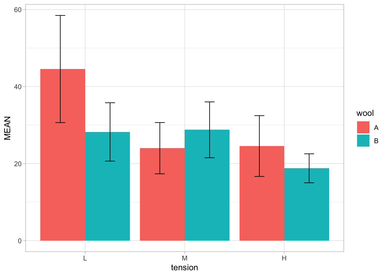
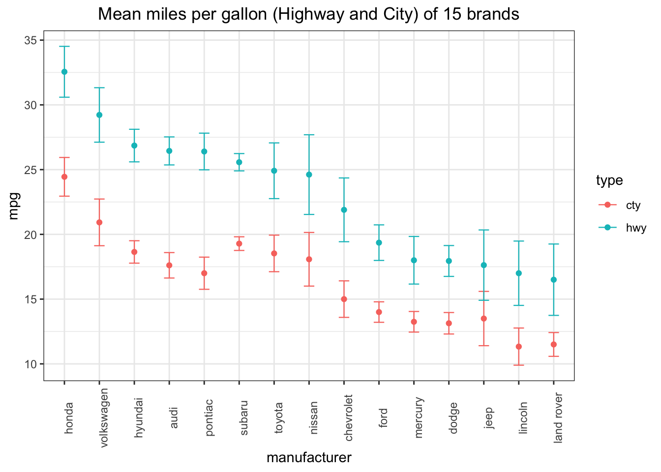
再用ggplot2中的mpg举一个例子:
mpg#> # A tibble: 234 x 11
#> manufacturer model displ year cyl trans drv cty hwy fl class
#> <chr> <chr> <dbl> <int> <int> <chr> <chr> <int> <int> <chr> <chr>
#> 1 audi a4 1.8 1999 4 auto… f 18 29 p comp…
#> 2 audi a4 1.8 1999 4 manu… f 21 29 p comp…
#> 3 audi a4 2 2008 4 manu… f 20 31 p comp…
#> 4 audi a4 2 2008 4 auto… f 21 30 p comp…
#> 5 audi a4 2.8 1999 6 auto… f 16 26 p comp…
#> 6 audi a4 2.8 1999 6 manu… f 18 26 p comp…
#> 7 audi a4 3.1 2008 6 auto… f 18 27 p comp…
#> 8 audi a4 q… 1.8 1999 4 manu… 4 18 26 p comp…
#> 9 audi a4 q… 1.8 1999 4 auto… 4 16 25 p comp…
#> 10 audi a4 q… 2 2008 4 manu… 4 20 28 p comp…
#> # … with 224 more rows你要如何根据manufacturer分组,查看每组中cty和hwy的平均值和标准误呢?自己尝试一下,然后对答案:
mpg_summary <- mpg %>% group_by(manufacturer) %>%
  summarise(n = n(),
            cty_mean = mean(cty),
            cty_SE = sd(cty)/sqrt(n),
            hwy_mean = mean(hwy),
            hwy_SE = sd(hwy)/sqrt(n))
mpg_summary
#> # A tibble: 15 x 6
#> manufacturer n cty_mean cty_SE hwy_mean hwy_SE
#> <chr> <int> <dbl> <dbl> <dbl> <dbl>
#> 1 audi 18 17.6 0.465 26.4 0.513
#> 2 chevrolet 19 15 0.671 21.9 1.17
#> 3 dodge 37 13.1 0.409 17.9 0.588
#> 4 ford 25 14 0.383 19.4 0.666
#> 5 honda 9 24.4 0.648 32.6 0.852
#> 6 hyundai 14 18.6 0.401 26.9 0.582
#> 7 jeep 8 13.5 0.886 17.6 1.15
#> 8 land rover 4 11.5 0.289 16.5 0.866
#> 9 lincoln 3 11.3 0.333 17 0.577
#> 10 mercury 4 13.2 0.25 18 0.577
#> 11 nissan 13 18.1 0.950 24.6 1.41
#> 12 pontiac 5 17 0.447 26.4 0.510
#> 13 subaru 14 19.3 0.244 25.6 0.309
#> 14 toyota 34 18.5 0.694 24.9 1.06
#> 15 volkswagen 27 20.9 0.877 29.2 1.02最终我们可以利用这些数据绘图(这将是下一章的练习):