1 Enzyme
2 ATP Synthase
3 Fluorescence spectroscopy
4 High-resolution Nuclear Magnetic Resonance Spectroscopy.
5 Electrospray mass spectrometry.
6 Analytical ultracentrifugation: equilibrium sedimentation.
\[ M = \dfrac{2RT}{(1-v\rho)\omega^2}\dfrac{d(\ln(c))}{dr^2} \]
\[ M = \dfrac{2\times 8.314\times298.15}{(1-0.74)\times27000^2}\dfrac{d(\ln(c))}{dr^2} = 2.6156\times10^{-5}\dfrac{d(\ln(c))}{dr^2} \]
r = c(6.918, 6.923, 6.924, 6.929, 6.932, 6.935, 6.942, 6.943, 6.945,
6.952, 6.955, 6.962, 6.964, 6.968, 6.973, 6.977, 6.978, 6.983,
6.985, 6.987, 6.992, 6.994, 6.998, 7.002, 7.004, 7.006, 7.009,
7.013, 7.016, 7.019, 7.022, 7.024, 7.026, 7.031, 7.033, 7.038,
7.042, 7.045, 7.047, 7.05, 7.053, 7.059, 7.061, 7.062, 7.065,
7.069, 7.07, 7.075, 7.077, 7.081, 7.084, 7.087, 7.09, 7.095,
7.098, 7.102, 7.106, 7.109, 7.11, 7.114, 7.116, 7.121, 7.123,
7.131, 7.137, 7.139, 7.141, 7.145, 7.146, 7.148, 7.15, 7.156,
7.158, 7.163, 7.166, 7.17)
od <- c(0.0645, 0.0658, 0.0731, 0.07, 0.0726, 0.0721, 0.0762, 0.0755,
0.0807, 0.082, 0.0809, 0.0914, 0.0909, 0.0969, 0.0979, 0.0983,
0.1054, 0.1038, 0.095, 0.1105, 0.1087, 0.1045, 0.1181, 0.1189,
0.1224, 0.1302, 0.1187, 0.133, 0.1306, 0.1413, 0.1378, 0.1371,
0.1333, 0.1521, 0.1481, 0.1578, 0.1498, 0.1495, 0.1605, 0.1699,
0.1664, 0.1757, 0.1802, 0.1834, 0.1882, 0.1856, 0.195, 0.2039,
0.1999, 0.1874, 0.2191, 0.2143, 0.215, 0.2186, 0.2283, 0.2347,
0.2677, 0.2532, 0.2596, 0.262, 0.2812, 0.271, 0.2816, 0.2841,
0.31, 0.3141, 0.3336, 0.3147, 0.334, 0.3528, 0.3548, 0.3572,
0.3752, 0.373, 0.3863, 0.3792)
Prepare data \(\ln(c)\) and \(r^2\):
# divide 2 by 100 to convert cm to m
r2 = (r/100)^2; lnc = log(od)
mod <- lm(lnc~r2)
summary(mod)##
## Call:
## lm(formula = lnc ~ r2)
##
## Residuals:
## Min 1Q Median 3Q Max
## -0.102145 -0.020829 0.001427 0.022606 0.074815
##
## Coefficients:
## Estimate Std. Error t value Pr(>|t|)
## (Intercept) -26.9712 0.2063 -130.7 <2e-16 ***
## r2 5065.5170 41.5559 121.9 <2e-16 ***
## ---
## Signif. codes: 0 '***' 0.001 '**' 0.01 '*' 0.05 '.' 0.1 ' ' 1
##
## Residual standard error: 0.03669 on 74 degrees of freedom
## Multiple R-squared: 0.995, Adjusted R-squared: 0.995
## F-statistic: 1.486e+04 on 1 and 74 DF, p-value: < 2.2e-16# only gradient is importantPlot it:
plot(r2, lnc)
abline(-26.9711515, 5065.51703)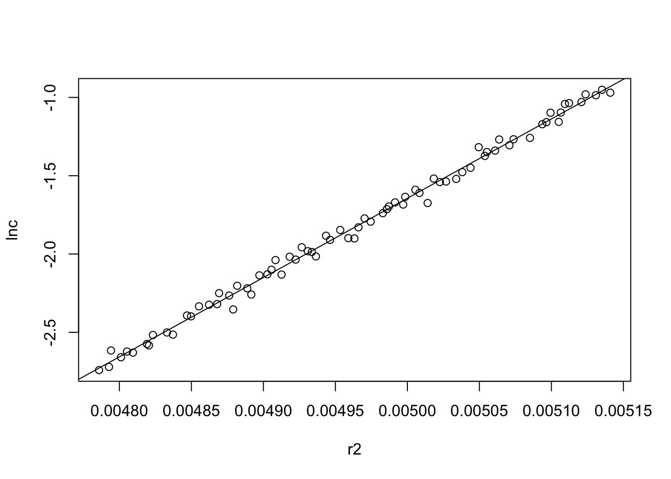
2.6156e-5 * 5065.51703## [1] 0.1324937#2.6156e-5 * 506551.703