How and why do proteins form specific complexes with each other? How can such protein-protein interactions (PPIs) be investigated experimentally, and which problems are associated with designing small molecules to disrupt PPIs?
1 Introduction
Specific protein-protein interactions (PPIs) are critical to numerous biological processes, including cell-cell recognition, immune response, and signal transduction. An understanding of PPIs not only helps to elucidate the detailed roles and to predict the behaviour of proteins in a physiological context but also aids structure-based drug design.
2 Properties of PPI
2.1 Reversibility
Protein-protein interactions can be stable (permanent) or transient. Stable interactions are involved in the assembly of proteins made of multi-subunit complexes such as haemoglobin, which non-reversible in normal physiological conditions. Transient interactions, on the other hand, are reversible, and it is this property that make them act like molecular switches that play versatile roles in controlling cellular processes.
2.2 Properties of the Binding Interfaces
Protein-protein interaction interfaces often have a large surface area (1000-2000 Å2) and are relatively flat compared to the deep cavities that typically bind small molecules. On a binding interface, some residues, known as “hotspots”, contribute to the overall affinity more than other residues.
2.3 Roles of Water Molecules
Crystal structures frequently reveal water molecules within PPI interfaces. These water molecules play multifaceted roles in the stability of PPI, e.g. offsetting unfavourable electrostatic interactions, bridging two distant residues via H-bonds.
2.4 Kinetics and Thermodynamics
Reversible PPIs have two important parameters: affinity and specificity. While affinity ranges from as low as millimolar to as high as femtomolar, it is important that the specificity, i.e. the relative affinity of a protein to its cognate binding partner compared to non-cognate ones, is high.
Reversible PPIs can the considered as a simple balance of association and dissociation reactions, with rate constants being \(k_{\text{on}}\) and \(k_{\text{off}}\).
\[ \text{A+B}\mathrel{\mathop{\rightleftarrows}^{k_{\text{on}}}_{k_{\text{off}}}} \text{AB} \]
The affinity is usually defined by the dissociation constant:
\[ K_\text{d} = \dfrac{\text{[A][B]}}{\text{[AB]}} = \dfrac{k_{\text{off}}}{k_{\text{on}}} \]
where [A], [B], and [AB] are the concentrations of each species at equilibrium.
\(K_\text{d}\) can be converted to \(\Delta G\) and vice versa:
\[ \Delta G = -RT\ln{(K_\text{d})} \]
In addition to the simple single-step model, Keeble and Kleanthous (2005) suggested that relatively low affinity PPIs may be better modelled with a two-step induced-fit mechanism involving an unstable intermediate, where electrostatics drives the fast first step (supported by strong dependence on ionic strength) and rigid body rotation occurs in the slow second step:
\[ \text{A+B} \mathrel{\mathop{\rightleftarrows}^{k_{1}}_{k_{-1}}} \text{AB}^\text{*} \mathrel{\mathop{\rightleftarrows}^{k_{2}}_{k_{-2}}} \text{AB} \]
3 Studying PPIs
3.1 Determining Kd (and rate constants)
Many experimental methods can be used used for studying thermodynamics and kinetics of PPIs (the frequent tasks are determining \(K_\text{d}\) and rate constants). Most of them assumes the simple single-step association-dissociation model (Section 2.4). Three methods are described in this essay.
3.1.1 Surface Plasmon resonance (SPR)
Surface plasmon resonance (Figure 3.1) can be used to measure both \(K_\text{d}\) and \(k_\text{on}\) and \(k_\text{off}\) rates. How \(K_\text{d}\) can be calculated is explained in Equation (3.1).
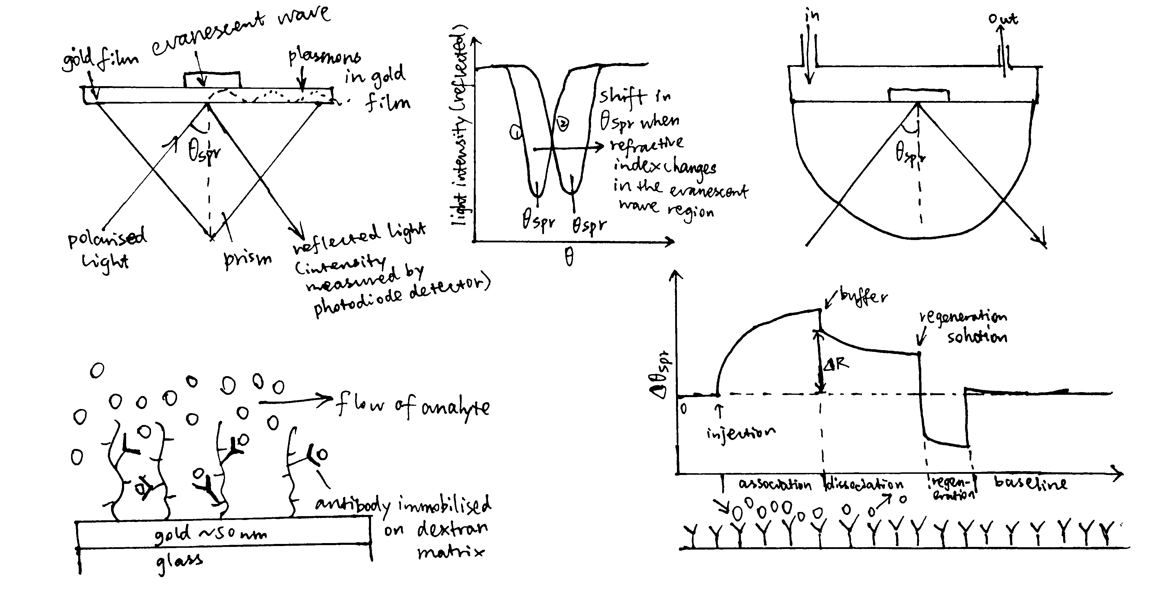
Figure 3.1: A surface plasmon is an electron oscillation generated at a surface interface between a metal and a dielectric. A plasmon resonance occurs when EM wave in visible light couples optimally with the oscillating electrons in the metal, and this results in a maximal reduction in the reflected light intensity. The resonance angle, \(\theta_\text{spr}\), is found by changing the angle of incidence of the light beam, giving a dip in a plot of intensity against angle. \(\Delta\theta_\text{spr}\) is sensitive to changes in the refractive index of the medium near the metal surface and this is a measure of the mass change at the sensor surface (in the evanescent region). In an SPR experiment, the protein acting as the “bait” is immobilised on the sensor surface, and a the analyte containing the other protein (acting as the “prey”) is passed through the cell. If binding occurs between the two proteins, \(\Delta\theta_\text{spr}\) would increase. Then, non-specific binding is washed off by buffer, and \(\Delta\theta_\text{spr}\) would decrease and \(\Delta\theta_\text{spr}\). Finally, regeneration solution is applied to remove all binding and reset \(\Delta\theta_\text{spr}\) to zero.
\[\begin{equation} \begin{split} \overbrace{k_{\text{on}}\text{[A][B]}}^\text{rate of association} & = \overbrace{k_{\text{off}}\text{[AB]}}^\text{rate of dissociation} \\ k_{\text{on}}\text{[A]([B]}_{\text{max}}-\text{[AB])} & = k_{\text{off}}\text{[AB]} \\ \text{[AB]} & = \dfrac{k_{\text{on}}\text{[A][B]}_{\text{max}}}{k_{\text{on}}\text{[A]} + k_{\text{off}}} \\ \text{[AB]} & = \dfrac{\text{[A][B]}_{\text{max}}}{\text{[A]} + K_{\text{d}}} \end{split} \tag{3.1} \end{equation}\]
In the equation, A is the protein in the analyte, whose concentration is kept constant, and B is the immobilised protein. Since the \(\Delta\theta_\text{spr} \propto \text{[AB]}\) (intensity of the signal is proportional to concentration of protein-protein complexes), we can work out \(K_\text{d}\) from our initial concentrations of A and B.
SPR was used in the early kinetic analysis of hGH binding (Wells (1996)).
3.1.2 Fluorescence anisotropy
Fluorescence anisotropy is based on the phenomenon that, if fluorophores are excited with plane polarized light and the fluorescence is observed through analyzing polarizers, the fluorescence is also polarised.
The fluorescence anisotropy is defined as \(A=\dfrac{I_\parallel - I_\bot}{I_\parallel+2_{\bot}}\), where \(I_\parallel\) and \(I_{\bot}\) are the fluorescence intensities polarised parallel and perpendicular to the direction of the excitation beam. \(A\) is a direct measure of the molecular rotation in solution and can be used to study complex formation, as a macromolecule will rotate more slowly when it is in a complex thatn when it is alone.
Fluorescence anisotropy is more accurate than SPR for measuring ultra-high affinity interactions, and were used to to study ColE DNase-Im interactions (Papadakos, Wojdyla, and Kleanthous (2012)).
3.1.3 Isothermal titration calorimetry (ITC)
ITC measures heat changes when a complex is formed at constant temperature. In ITC, an insulated reaction cell containing protein is kept at a temperature (usually 8\(^\circ\text{C}\) above the environment) which is equal to the temperature of a reference cell, and the reference cell is kept at a constant temperature by a thermostat. Then, increasing amounts of ligand is added into the chamber, and they form complexes with the protein, which can be exothermic or endothermic. The heat change is compensated by a power supply, which can be converted to \(\Delta H\) of the reaction. As more ligands are added, proteins become saturated and \(\Delta H\) approaches zero. The raw data obtained (power supplied to compensate the heat change caused by each addition of ligands) can be integrated and corrected to give a plot of \(\Delta H\) against the molar ratio of the ligand and the protein, and \(\Delta H\), Kd and stoichiometry can be inferred from the curve (Figure 3.2).
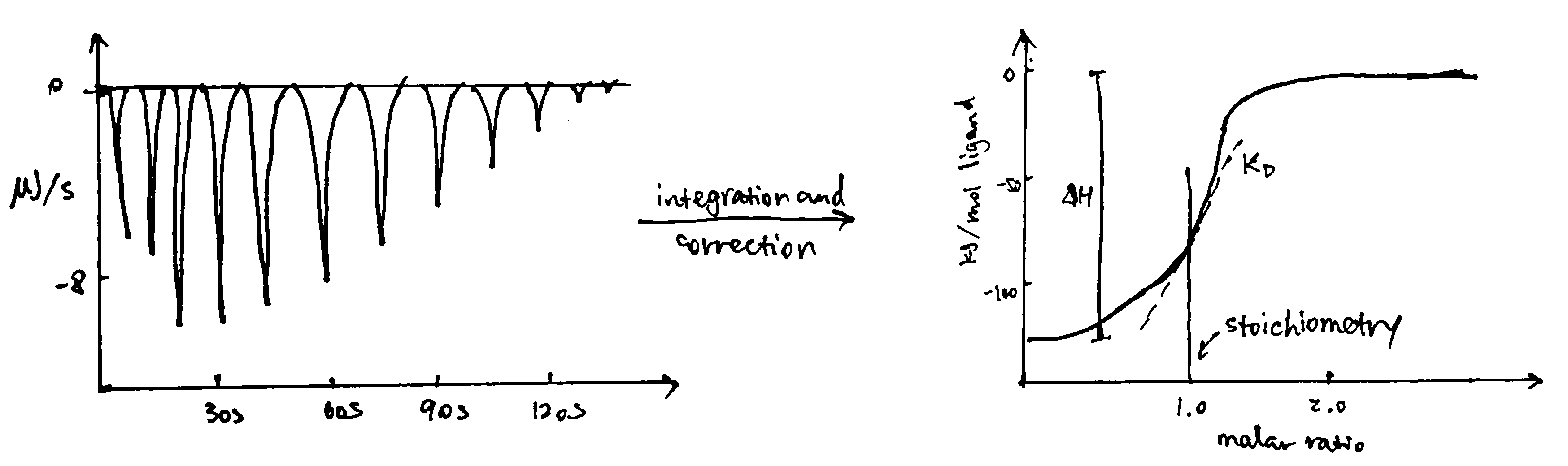
Figure 3.2: ITC data manipulation
3.2 Mechanistic Studies
The main theme of mechanistic studies is to find out the “hotspot” residues or regions that are main contributors to the affnity of PPI interfaces, and to attempt to generalise this knowledge in order to predict the affnity of any given PPI interfaces.
3.2.1 Alanine Scanning
Alanine scanning is a mutagenesis technique in which mutants are made by substituting alanine for each of the residues in a ‘reactive region’, in this case the PPI interface. By comparing the PPI affininy of each mutant to the wild type (i.e. calculating \(\Delta \Delta G\)), the contribution of each residue in binding can be assessed, and this reveals “hotspots” representing important residues.
3.2.2 Extent of Exchengeability of Amino Acids
Mutational analysis is most often restricted to alanine substitution and this does not provide an comprehensive view of the allowed amino acid space at each position. This limitation is especially significant in the analysis of PPI interfaces, which, unlike enzyme active sites, the specific orientation and chemical reactivity are less important.
Pál et al. (2006) introduced any one of the 20 natrual amino acids at all 35 hGH-hGHR binding interface positions and obtained surprising results. They verified that, the interface was highly adaptable to mutations, either from a structural or functional point of view. Whereas some of the alanine scanning hotspots showed high specificity agianst substitution, others did not, and some highly specific positions were not hotspots at all.
3.2.3 Directed Evolution
Directed evolution is an efficient approach to probe sequence and structure space in a PPI. Phage display is a specific implementation of it.
The phage display technique is summarised as follows and illustrated in Figure 3.3:
- Generate a randomised library of mutants. This can be done using error-prone PCR (ep-PCR). In PPI studies usually the randomised mutations are generated only across small sections of protein sequence that are form of the PPI interface.
- The randomised mutant DNA are ligated with a phage coat protein gene and the hybrid is then used to transduce E. coli. cells.
- The phage library is amplified by E. coli. cells, and phage particles are produced.
- The “bait” protein is immobilised, and the mixture of phage particles displaying different mutant proteins are added. Then, those with low binding affinity are washes away, and the remaining phages and collected, amplified, and used in the next round of selection.
- Repeated cycles of selection (a.k.a. “panning”) will identify the mutant proteins with the highest binding affinity to the “bait” protein. The complexes formed by these proteins with the “bait” protein can then be used for detailed mechanistic studies of PPI.
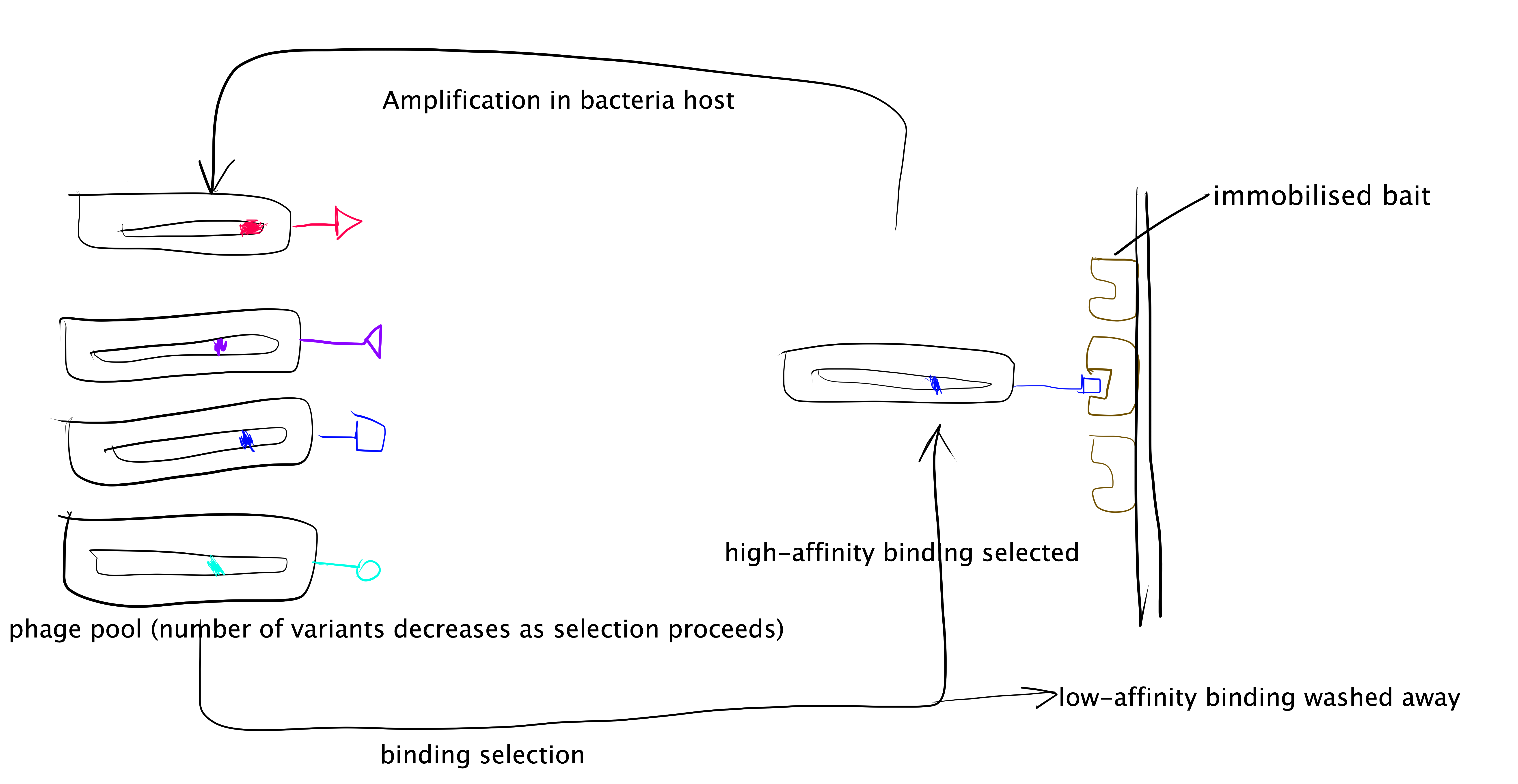
Figure 3.3: Directed evolution with phage display.
3.2.4 Computational Approaches
Computational methods can speed up the quest for high-affinity PPIs. These methods are based on rotamer libraries, which summarise the existing knowledge of the experimentally determined structures quantitatively. Rotamers are picked from the library (hotspot constraints may be applied) and grafted onto the scaffold of known structure, then the fitness is assessed using a scoring function, which unfortunately often fails to predict the actual experimental results. As the number rotamers in the library grows and algorithms improve, computational methods are expected to provide more accurate predictions.
3.2.5 Connectivity Map Reveals Modularity
Reichmann et al. (2005) analysed the TEM1–BLIP complex by drawing a connectivity map, which is build from the physical interactions between the proteins (hydrogen bonds, van der Waals interactions, etc.), and showed that the interface can be divided into 6 clusters. The change \(\Delta \Delta G\) on different clusters was found to be additive, whereas mutations within the same cluster caused complex energetic and structural consequences. Therefore, a PPI interface can be seen as a group of “hot regions”, where each region contribute relatively independently to the total binding affinity, but within each region the contributions from its component amino acids are cooperative.
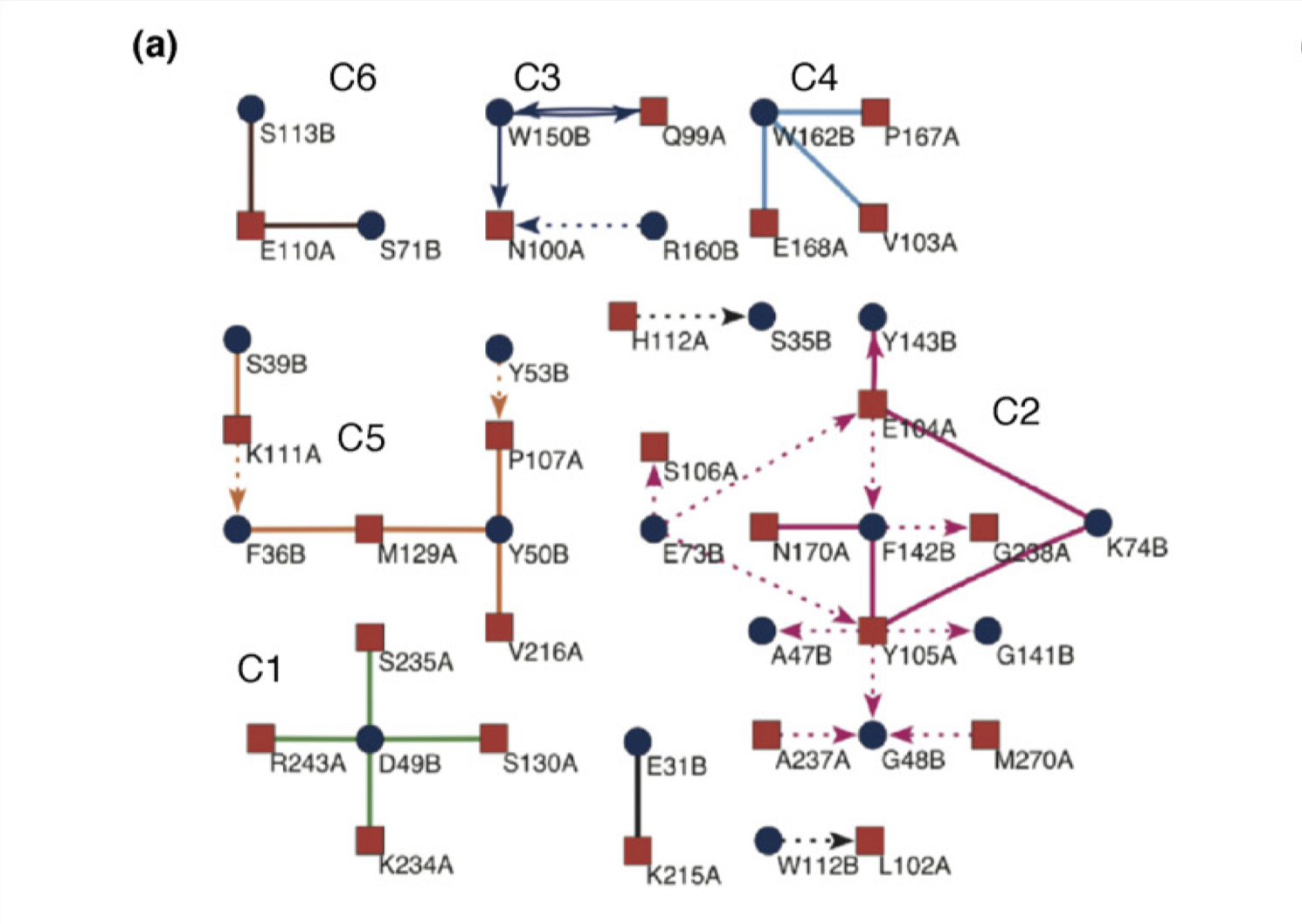
Figure 3.4: Connectivity map of the TEM1–BLIP complex.
3.2.6 X-Ray Crystallography
X-ray crystallography (XRC) studies provide structural basis for PPI interfaces, which not only facilitates the analysis of individual cases but also help to improve the scoring algorithms for computational methods.
Crystallisation tends to be difficult for low affnity PPIs due to their unstable nature. To overcome this, correctly positioned cysteines can be introduced into each of the binding partners at the interface, which could stabilise the complex, facilitating crystallisation. This technique is known as “disulfide trapping”.
4 Why Designing Small Molecule PPI Inhibitors is Difficult
PPI interfaces are usually large and flat (Section 2.2), and often tolerent to a small number of mutations (Section 3.2.2). Thus, the “druggable” targets are usually restricted to the local non-flat regions (i.e. ‘pockets’) on PPI interfaces that are enriched with “hotspot” residues. A large surface area of PPI interface, which is more tolerent to local non-favourable interactions, also makes developing inhibitors more difficult. In addition, in the case of developing non-peptide inhibitors, there is less existing knowledge on the structures of small molecules and their interactions with proteins, meaning the computational modelling is less accurate.
References
Arkin, Michelle R, Yinyan Tang, and James A Wells. 2014. “Small-Molecule Inhibitors of Protein-Protein Interactions: Progressing Toward the Reality.” Chem Biol 21 (9): 1102–14. https://doi.org/10.1016/j.chembiol.2014.09.001.
Keeble, Anthony H, and Colin Kleanthous. 2005. “The Kinetic Basis for Dual Recognition in Colicin Endonuclease-Immunity Protein Complexes.” J Mol Biol 352 (3): 656–71. https://doi.org/10.1016/j.jmb.2005.07.035.
Papadakos, Grigorios, Justyna A. Wojdyla, and Colin Kleanthous. 2012. “Nuclease Colicins and Their Immunity Proteins.” Quarterly Reviews of Biophysics 45 (1): 57–103. https://doi.org/10.1017/S0033583511000114.
Pál, Gábor, Jean-Louis K Kouadio, Dean R Artis, Anthony A Kossiakoff, and Sachdev S Sidhu. 2006. “Comprehensive and Quantitative Mapping of Energy Landscapes for Protein-Protein Interactions by Rapid Combinatorial Scanning.” J Biol Chem 281 (31): 22378–85. https://doi.org/10.1074/jbc.M603826200.
Reichmann, D, O Rahat, S Albeck, R Meged, O Dym, and G Schreiber. 2005. “The Modular Architecture of Protein-Protein Binding Interfaces.” Proc Natl Acad Sci U S A 102 (1): 57–62. https://doi.org/10.1073/pnas.0407280102.
Wells, J A. 1996. “Binding in the Growth Hormone Receptor Complex.” Proceedings of the National Academy of Sciences 93 (1): 1–6. https://doi.org/10.1073/pnas.93.1.1.
Wienken, Christoph J., Philipp Baaske, Ulrich Rothbauer, Dieter Braun, and Stefan Duhr. 2010. “Protein-Binding Assays in Biological Liquids Using Microscale Thermophoresis.” Nature Communications 1 (1): 100. https://doi.org/10.1038/ncomms1093.