1 Aim
- Given a sample containing (fake) radioactive 14C glucose and 3H ATP:
- determine concentration of glucose and ATP.
- Given that both concentrations lie between 1mM and 10mM.
- Given that \(\epsilon^{260}_\text{ATP}=1.57\times10^4 \text{ mol}^{-1}\text{ dm}^3\text{ dm}^{-1}\)
- determine radioactivity of the sample (virtual practical)
- and hence determine the specific radioactivity of ATP and glucose
- determine concentration of glucose and ATP.
- 23 samples have glucose and ATP concentrations falling into two distinct classes. They are independently measured by 23 pairs of students. Determine these concentrations using the class results and assess precision and accuracy.
2 Reagents and Apparatus Provided
- 15mL sample solution
- 0.1 M Na3PO4 buffer at pH 7.0
- 1mM ABTS
- Glucose Oxidase (100 U/mL) and peroxidase (20 U/mL)
- Solid glucose
- Spectrophotometer
3 Method
3.1 ATP concentration
3.1.1 Dilution
3.1.1.1 Determining scale of dilution
Given that 1mM < ATP < 10mM and that \(\epsilon^{260}_\text{ATP}=1.57\times10^4 \text{ mol}^{-1}\text{ dm}^3\text{ dm}^{-1}\), according to \(A^{260}=\epsilon^{260}cl\):
if no dilution:
\[ \begin{aligned} 1.57\times10^4\times0.001<&A^{260}<1.57\times10^4\times0.01 \\ 15.7<&A^{260}_\text{raw}<157 \\ \end{aligned} \]
clearly, a 1:100 dilution would be very likely to produce a sensible \(A^{260}\):
\[0.157<A^{260}_\text{1:100 dilution}<1.57\]
3.1.1.2 Making dilution
5mL of 1:100 diluton is made serially by first fixing 500 \(\mu\text{L}\) sample with 4.5mL buffer then mixing 500 \(\mu\text{L}\) of the resulting 1:10 dilution with another 4.5mL buffer.
A preliminary test gives \(A^{260}_\text{1:100 dilution}=0.503\), which is within the range where the spectrophotometer is accurate, so we made 4 more 1:100 dilutions using the method described above.
3.1.2 Results
See section 4.1
3.2 Glucose concentration
3.2.1 Mechanism
Glucose itself does not have convenient absorption. Thus, glucose oxidase, ABTS and peroxidase is added to make a green solution (glucose is first oxidised by oxidase to produce gluconic acid and H2O2; peroxidase then catalyses the reaction between H2O2 and ABTS to produce a green dye).
3.2.2 Determine the volume of enzyme
We want the reaction to ‘virtually’ complete (i.e. > 99% conversion of substrate) in 10 min.
For an enzyme reaction:
\[-\dfrac{ds}{dt}=v-\dfrac{V_\text{max}s}{K_m+S}\]
As the reaction approaches completion, \(s<<K_m\):
\[-\dfrac{ds}{dt}=\dfrac{V_\text{max}s}{K_m}\]
Integrating to determine the total time for a given change in \(s\):
\[ \begin{aligned} -\int_{s_0}^{s_1}{\dfrac{ds}{s}}&=\dfrac{V_\text{max}}{K_m}\int_0^t dt \\ \ln\dfrac{s_0}{s_1}&=\dfrac{V_\text{max}t}{K_m} \end{aligned} \]
For a decrease in \(s\) from 100% to 1% in 10 min:
\[ \begin{aligned} \ln\dfrac{100}{1}&=\dfrac{V_\text{max}\times 10}{K_m} \\ V_\text{max}&=0.4605K_m \text{ (mol L}^{-1}\text{min}^{-1}\text{)} \end{aligned} \]
Our assay volume will be 4.0mL, so the amound of enzyme, in U (\(\mu\text{mol min}^{-1}\)), will be
\[\text{amount of enzyme in U}=0.4605\times K_m \times 4.0 \times 10^{-3}\times10^6=1842K_m\]
where \(K_m\) has unit M.
For GOD, \(K_m=1\text{ mM}\), and the provided enzyme concentration is 100U/mL:
\[ \begin{aligned} K_m&=1\text{ mM} \\ \text{minimum amount of enzyme}&=1842 \times 1 \times 10^{-3}=1.84 \text{ U} \\ \text{minimum volume of enzyme}&=1.84 \div 100=0.0184 \text{ mL} \end{aligned} \]
For POD, \(K_m=100\text{ }\mu\text{M}\), and the provided enzyme concentration is 20U/mL:
\[ \begin{aligned} K_m&=100\text{ }\mu\text{M} \\ \text{minimum amount of enzyme}&=1842 \times 100 \times 10^{-6}=0.184 \text{ U} \\ \text{minimum volume of enzyme}&=0.184 \div 20=0.0092 \text{ mL} \end{aligned} \]
We decided to use an excess amount of enzyme (i.e. 0.1mL for both). This guarantees that the reactions will complete within 10 min, and makes it easier to make up the 4mL total volume for assay (see section 3.2.4.2).
3.2.3 Determining \(\lambda_\text{max}\)
Measuring absorbance near \(\lambda_\text{max}\) reduces error. An 100nmol-glucose-containing (i.e. with 1mL 0.1mM glucose solution, see section 3.2.4.2) assay result is used. The absorbance in the range 350nm to 450nm is measured, and \(\lambda_\text{max} = 418\text{ nm}\). We then used this wavelength for all glucose assays.
3.2.4 Calibration
Calibrate \(A^{418}\) with known glucose concentrations, then we can map \(A^{418}_\text{sample}\) to the calibration curve to determine sample glucose concentration.
3.2.4.1 Dilution
- 0.18 g glucose is dissolved in 100mL buffer, which gives 10mM glucose solution (which is handy, as the maximum possible concentration of glucose in the sample is also 10mM)
- 100mL 0.1mM glucose solution is made by mixing 1mL 10mM glucose solution with 99mL buffer (1:100 dilution).
3.2.4.2 Assay
Assays are made on 4mL mixtures with varying amount of glucose, according to the following table:
| ABTS | Buffer | 0.1mM glucose | H2O | GOD | POD | nmol glucose |
|---|---|---|---|---|---|---|
| 2mL | 0.8mL | 1.0mL | 0mL | 0.1mL | 0.1mL | 100 |
| 2mL | 0.8mL | 0.8mL | 0.2mL | 0.1mL | 0.1mL | 80 |
| 2mL | 0.8mL | 0.6mL | 0.4mL | 0.1mL | 0.1mL | 60 |
| 2mL | 0.8mL | 0.4mL | 0.6mL | 0.1mL | 0.1mL | 40 |
| 2mL | 0.8mL | 0.2mL | 0.8mL | 0.1mL | 0.1mL | 20 |
| 2mL | 0.8mL | 0mL | 1.0mL | 0.1mL | 0.1mL | 0 |
Then the mixture is incubated at 37\(^\circ\text{C}\) for 10 minutes (in a theromostatically-controlled water bath), then \(A^{418}\) is measured.
Every row is repeated 3 times.
3.2.5 Sample Assay
The sample is diluted 1:100 by mixing 1mL sample with 99mL buffer.
4mL assays are made on 1mL 1:100 dilution 3 times, according to the following table (identical to the assays used for calibration except that an unknown concentration is used this time)
| ABTS | Buffer | diluted sample | GOD | POD | |
|---|---|---|---|---|---|
| 2mL | 0.8mL | 1.0mL | 0.1mL | 0.1mL |
3.2.6 Results
See section 4.2
3.3 Radioactivity Counting (Virtual)
0.2mL sample is mixed with 1.8mL scintillation fluid in a polyvial and placed into the scintillation counter. The count time is 2min. The results are shown in section 5.5.
4 Our Results
4.1 ATP
(Methods in section 3.1)
A <- c(0.503, 0.513, 0.508, 0.525, 0.516)
c_ATP <- A/1.57e4*100*1000
kable(tibble(`$A^{260}_\\text{1:100 dilution}$`=A, `[ATP] of raw sample (mM)`=c_ATP))| \(A^{260}_\text{1:100 dilution}\) | ATP of raw sample (mM) |
|---|---|
| 0.503 | 3.203822 |
| 0.513 | 3.267516 |
| 0.508 | 3.235669 |
| 0.525 | 3.343949 |
| 0.516 | 3.286624 |
Statistical summary of ATP in sample:
x <- c_ATP; n <- length(x); df <- n - 1; t = qt(0.975, df)
c(mean=mean(x), sd=sd(x), SE=sd(x)/sqrt(n), t = t, `t*SE` = t*sd(x)/sqrt(n))
## mean sd SE t t*SE
## 3.26751592 0.05309978 0.02374695 2.77644511 0.06593209Which gives 95% confidence interval: \(\text{[ATP]}=3.268\pm0.054\) mM
4.1.1 Distinguishing between 4.0mM and 4.5mM ATP
The percentage error (coefficient of variance) of this experiment is:
\[c_v=\dfrac{s_x}{\bar{x}}=\dfrac{0.054}{3.268}=0.0165\]
for \(\bar{x}\) = 4.0 and 4.5, \(s_x=c_v\bar{x}\) = 0.0661 and 0.0744, respectively.
To distinguish between the two, two sample t test is used. If \(n\) measurements are made on each concentration, then
\[t=\dfrac{\bar{x_1}-\bar{x_2}}{\sqrt{\dfrac{s_1^2}{n}+\dfrac{s_2^2}{n}}}=\dfrac{4.5-4.0}{\sqrt{\dfrac{0.0661^2+0.0744^2}{n}}}=\sqrt{25.26n}\]
then we can get a list of \(p\) values for each \(n\):
n <- 2:8
df <- n - 1
t <- sqrt(25.26 * n)
p <- (1 - pt(t, df)) * 2
names(p) <- paste('n =', n)
round(p, 5)
## n = 2 n = 3 n = 4 n = 5 n = 6 n = 7 n = 8
## 0.08898 0.01294 0.00210 0.00036 0.00006 0.00001 0.00000as n increases, \(p\) decreases. When n = 3, \(p\) is already less than 0.05.
4.2 Glucose
(Methods in section 3.2)
4.2.1 Calibration
The results are shown below:
A1 <- c(0.952, 0.815, 0.709, 0.496, 0.272, 0)
A2 <- c(1.223, 0.969, 0.704, 0.415, 0.222, 0)
A3 <- c(1.194, 0.919, 0.682, 0.452, 0.236, 0)
A <- c(A1, A2, A3)
glucose = c(100, 80, 60, 40, 20, 0)
kable(tibble(`nmol glucose in 4mL assay` = glucose, `$A^{418}_1$` = A1,
`$A^{418}_2$` = A2, `$A^{418}_3$` = A3))| nmol glucose in 4mL assay | \(A^{418}_1\) | \(A^{418}_2\) | \(A^{418}_3\) |
|---|---|---|---|
| 100 | 0.952 | 1.223 | 1.194 |
| 80 | 0.815 | 0.969 | 0.919 |
| 60 | 0.709 | 0.704 | 0.682 |
| 40 | 0.496 | 0.415 | 0.452 |
| 20 | 0.272 | 0.222 | 0.236 |
| 0 | 0.000 | 0.000 | 0.000 |
To fit a straight line, linear regression is used. The coefficients are shown below:
summary(lm(A ~ 0 + rep(glucose, 3)))##
## Call:
## lm(formula = A ~ 0 + rep(glucose, 3))
##
## Residuals:
## Min 1Q Median 3Q Max
## -0.181273 -0.000982 0.005691 0.039277 0.089727
##
## Coefficients:
## Estimate Std. Error t value Pr(>|t|)
## rep(glucose, 3) 0.0113327 0.0002387 47.48 <2e-16 ***
## ---
## Signif. codes: 0 '***' 0.001 '**' 0.01 '*' 0.05 '.' 0.1 ' ' 1
##
## Residual standard error: 0.06132 on 17 degrees of freedom
## Multiple R-squared: 0.9925, Adjusted R-squared: 0.9921
## F-statistic: 2254 on 1 and 17 DF, p-value: < 2.2e-16which shows there is a linear relationship \(A^{418}=0.01133n_\text{glucose}\) with \(R^2=0.9921\).
Then we can plot it (CI added).
ggplot(data.frame(A, glucose), aes(glucose, A))+
  geom_point()+
  geom_smooth(formula = y ~ 0 + x, method = 'lm')+
  labs(x = 'nmol glucose in 4mL assay', y = expression(A ^ 418),
       title = 'Calibrationn Curve for 4mL essay')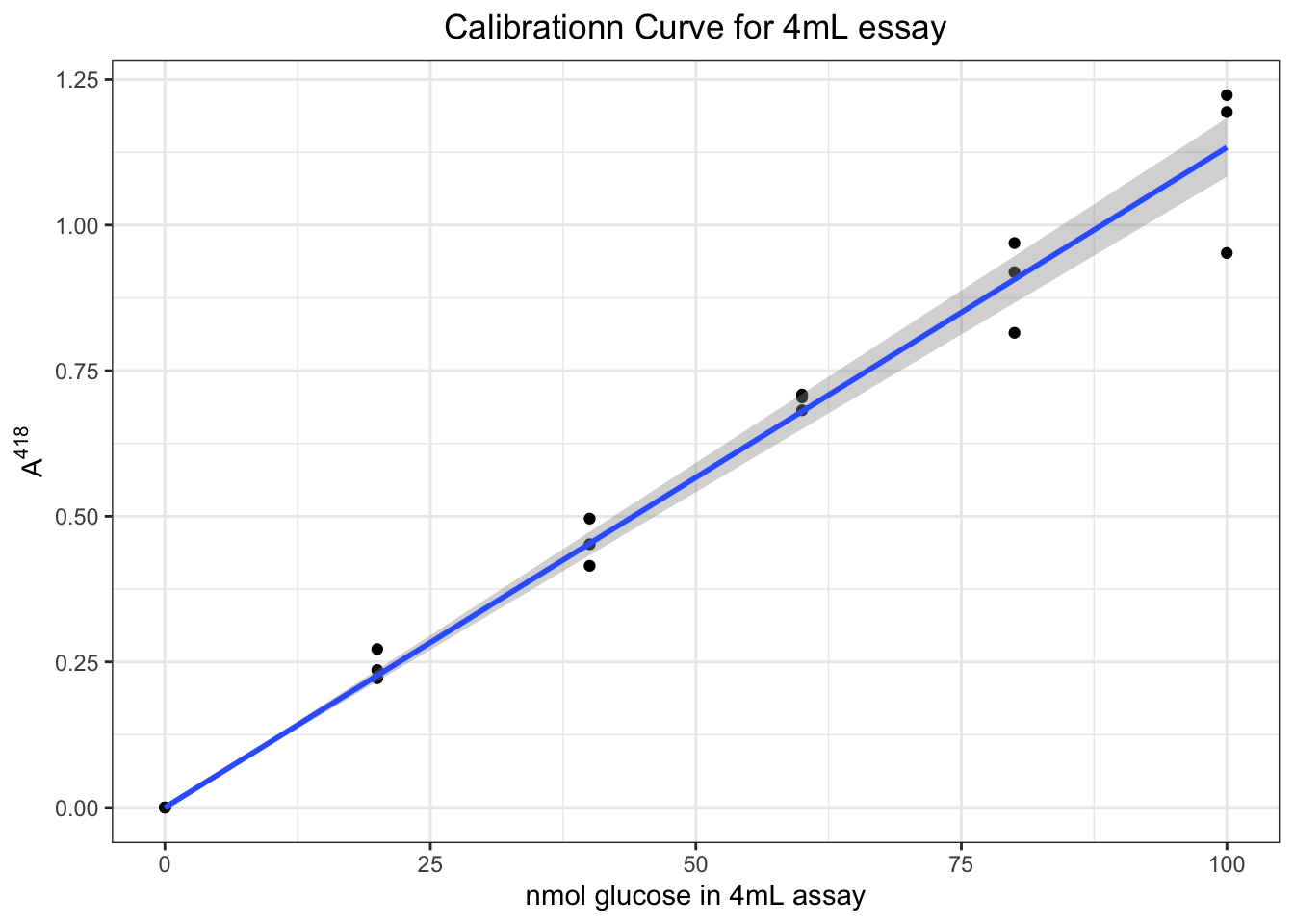
4.2.2 Sample result
Three independent measurements of \(A^{418}_\text{sample}\) gives 0.863, 0.872 and 0.871. According to the linear relationship \(A^{418}=0.01133n_\text{glucose}\) we can calculate the amount (in nmol) of glucose in 1mL 1:100 dilution, then the concentration of the raw sample can be calculated easily:
A <- c(0.863, 0.872, 0.871) # sample absorbance
n <- A/0.01133 # nmol glucose in 1 mL 1:100 dilution
(c_glucose_sample <- n * 1e-9 # converting to mol/mL (1:100 dilution)
       / 1e-3 # converting to M (1:100 dilution)
       * 100 # in M (raw sample)
       * 1e3) # converting to mM (raw sample)
## [1] 7.616946 7.696381 7.687555Statistical summary:
x <- c_glucose_sample; n <- length(x); df <- n - 1; t = qt(0.975, df)
c(mean=mean(x), sd=sd(x), SE=sd(x)/sqrt(n), t = t, `t*SE` = t * sd(x)/sqrt(n))
## mean sd SE t t*SE
## 7.66696087 0.04353824 0.02513682 4.30265273 0.10815499Which gives 95% confidence interval: \(\text{[glucose]}=7.667\pm0.057\) mM
4.2.3 Distinguishing between 4.0mM and 4.5mM glucose
Similar to the calculation for ATP shown in section 4.1.1, first calculate the percentage error (coefficient of variance) of this experiment:
\[c_v=\dfrac{s_x}{\bar{x}}=\dfrac{0.057}{7.667}=0.00743\]
for \(\bar{x}\) = 4.0 and 4.5, \(s_x=c_v\bar{x}\) = 0.0297 and 0.0335, respectively.
To distinguish between the two, two sample t test is used. If \(n\) measurements are made on each concentration, then
\[t=\dfrac{\bar{x_1}-\bar{x_2}}{\sqrt{\dfrac{s_1^2}{n}+\dfrac{s_2^2}{n}}}=\dfrac{4.5-4.0}{\sqrt{\dfrac{0.0297^2+0.0335^2}{n}}}=\sqrt{124.7n}\]
then we can get a list of \(p\) values for each \(n\):
n <- 2:8
df <- n - 1
t <- sqrt(124.7 * n)
p <- (1 - pt(t, df)) * 2
names(p) <- paste('n =', n)
round(p, 5)
## n = 2 n = 3 n = 4 n = 5 n = 6 n = 7 n = 8
## 0.04026 0.00266 0.00020 0.00002 0.00000 0.00000 0.00000as n increases, \(p\) decreases. When n = 2, \(p\) is already less than 0.05.
4.2.3.1 What difference would it make to your assay if you doubled the concentrations of ABTS, GOD and POD?
Time required for incubation will be shorter and the final intensity of colors (and hence absorption) will be the same.
5 Class Results
5.1 Data1
ATP <- c(3.93, 4.04, 3.01, 3.94, 3.20, 3.15, 2.81,
         4.07, 3.17, 3.05, 4.20, 3.15, 4.17, 3.05,
         3.90, 2.97, 3.11, 4.13, 3.27, 3.85, 2.92)
ATP_sd <- c(0.164, 0.082, 0.080, 0.080, 0.140, 0.126, 0.139,
            0.071, 0.140, 0.142, 0.002, 0.012, 0.240, 0.033,
            0.051, 0.091, 0.187, 0.160, 0.053, 5.e-4, 0.218)
glucose <- c(6.89, 6.92, 8.36, 7.38, 7.10, 7.65, 7.70,
             9.09, 7.34, 7.60, 8.92, 8.80, 8.50, 6.60,
             3.81, 9.80, 7.73, 9.80, 7.67, 8.50, 8.63)
glucose_sd <- c(0.0880, 0.0104, 0.1560, 0.0150, 0.0603, 0.5900, 1.4580,
                0.0470, 0.1640, 0.2810, 0.2500, 0.2000, 0.0010, 0.1180,
                0.0170, 0.0425, 0.1500, 0.0530, 0.0440, 0.1400, 0.4800)
class_results <- tibble(ATP, ATP_sd, glucose, glucose_sd)
kable(tibble(`ATP conc`=ATP, `ATP sd`=ATP_sd,
`Glucose conc`=glucose, `Glucose sd`=glucose_sd))| ATP conc | ATP sd | Glucose conc | Glucose sd |
|---|---|---|---|
| 3.93 | 0.1640 | 6.89 | 0.0880 |
| 4.04 | 0.0820 | 6.92 | 0.0104 |
| 3.01 | 0.0800 | 8.36 | 0.1560 |
| 3.94 | 0.0800 | 7.38 | 0.0150 |
| 3.20 | 0.1400 | 7.10 | 0.0603 |
| 3.15 | 0.1260 | 7.65 | 0.5900 |
| 2.81 | 0.1390 | 7.70 | 1.4580 |
| 4.07 | 0.0710 | 9.09 | 0.0470 |
| 3.17 | 0.1400 | 7.34 | 0.1640 |
| 3.05 | 0.1420 | 7.60 | 0.2810 |
| 4.20 | 0.0020 | 8.92 | 0.2500 |
| 3.15 | 0.0120 | 8.80 | 0.2000 |
| 4.17 | 0.2400 | 8.50 | 0.0010 |
| 3.05 | 0.0330 | 6.60 | 0.1180 |
| 3.90 | 0.0510 | 3.81 | 0.0170 |
| 2.97 | 0.0910 | 9.80 | 0.0425 |
| 3.11 | 0.1870 | 7.73 | 0.1500 |
| 4.13 | 0.1600 | 9.80 | 0.0530 |
| 3.27 | 0.0530 | 7.67 | 0.0440 |
| 3.85 | 0.0005 | 8.50 | 0.1400 |
| 2.92 | 0.2180 | 8.63 | 0.4800 |
5.2 Preliminary graphical analysis
Density plots and histograms are used to examine the distribution of measurements:
op <- par(mfrow=c(2,2))
for(i in c('ATP', 'glucose')){
  main = paste0('[', i, '] in 21 samples:'); xlab <- paste(i, 'concentration')
  {
    plot(density(class_results[[i]], bw = c(ATP = 0.1, glucose = 0.2)[i]),
         main = paste(main, 'density plot'), xlab = xlab)
    rug(class_results[[i]])
  }
  {
    hist(class_results[[i]], breaks = 10, main = paste(main, 'histogram'), xlab = xlab)
  }
}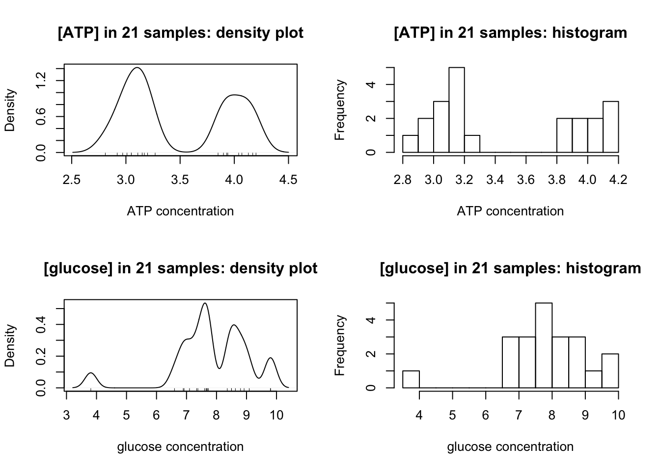
Clealy, ATP has a clear bimodal distribution, with two peaks at around 3.1 and 4.0.
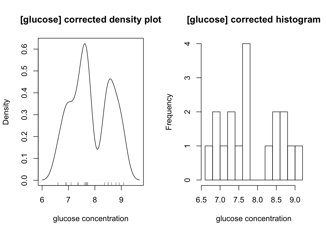
The distibution of glucose is affected by two outliers (the maximum and minimum). After their removal, a bimodal distribution, which peaks at 7.6 and 8.8, is also produced:
op <- par(mfrow=c(1,2))
glucose <- glucose[glucose != max(glucose) & glucose != min(glucose)]
main = '[glucose] corrected'; xlab <- 'glucose concentration'
{
  plot(density(glucose, bw = c(ATP = 0.1, glucose = 0.2)[i]),
       main = paste(main, 'density plot'), xlab = xlab)
  rug(glucose)
}
{
  hist(glucose, breaks = 10, main = paste(main, 'histogram'), xlab = xlab)
}
5.3 ATP concentration
5.3.1 Grouping and grouped confidence interval of mean
According to the plots, evidently there are two ATP concentrations, so we need to divide the 21 measurements into two groups, and calculate their mean and CI separately.
ATP1 <- ATP[ATP < 3.5] # less than 3.5mM, around 3.0mM
ATP2 <- ATP[ATP > 3.5] # more than 3.5mM, around 4.0mM
For the ATP around 3.0:
x <- ATP1; n <- length(x); df <- n - 1; t = qt(0.975, df)
c(mean=mean(x), sd=sd(x), SE=sd(x)/sqrt(n), t = t, `t*SE` = t*sd(x)/sqrt(n))
## mean sd SE t t*SE
## 3.07166667 0.12995337 0.03751431 2.20098516 0.0825684395% confidence interval: \(\text{[ATP]}=3.07\pm0.08\) mM
For the ATP around 4.0:
x <- ATP2; n <- length(x); df <- n - 1; t = qt(0.975, df)
c(mean=mean(x), sd=sd(x), SE=sd(x)/sqrt(n), t = t, `t*SE` = t*sd(x)/sqrt(n))
## mean sd SE t t*SE
## 4.02555556 0.12620530 0.04206843 2.30600414 0.0970099895% confidence interval: \(\text{[ATP]}=4.03\pm0.10\) mM
5.3.2 Test for significance of the difference in concentration between the two groups
To test there is a significant difference between the two concentrations, t-test2 is used:
t.test(ATP1, ATP2)##
## Welch Two Sample t-test
##
## data: ATP1 and ATP2
## t = -16.923, df = 17.66, p-value = 2.346e-12
## alternative hypothesis: true difference in means is not equal to 0
## 95 percent confidence interval:
## -1.0724720 -0.8353058
## sample estimates:
## mean of x mean of y
## 3.071667 4.025556\(p=2.3\times10^{-12}<<0.05\); the two concentrations are significantly different
5.3.3 Test for diviation from given concentrations
The solutions were actually made up to be 3.0mM and 4.0mM ATP. Were they made up correctly? We need two one-sample t tests using the given concentrations as the population mean, \(\mu\):
3.0mM: (\(H_0\): true concentration is 3.0mM)
t.test(ATP1, mu=3.0)##
## One Sample t-test
##
## data: ATP1
## t = 1.9104, df = 11, p-value = 0.08249
## alternative hypothesis: true mean is not equal to 3
## 95 percent confidence interval:
## 2.989098 3.154235
## sample estimates:
## mean of x
## 3.071667\(p=0.082>0.05\), failed to reject hypothesis. Solution made up correctly.
4.0mM: (\(H_0\): true concentration is 4.0mM)
t.test(ATP2, mu=4.0)##
## One Sample t-test
##
## data: ATP2
## t = 0.60748, df = 8, p-value = 0.5604
## alternative hypothesis: true mean is not equal to 4
## 95 percent confidence interval:
## 3.928546 4.122566
## sample estimates:
## mean of x
## 4.025556\(p=0.56>0.05\), failed to reject hypothesis. Solution made up correctly.
5.4 Glucose
5.4.1 Grouping and grouped confidence interval of mean
By observing the plots, the boundary between the two concentrations of glucose is 8.0mM, so we can divide them into two groups:
glucose1 <- glucose[glucose < 8.0]
glucose2 <- glucose[glucose > 8.0]
And calculate their 95% CIs separately:
lapply(list(glucose1=glucose1, glucose2=glucose2), function(x){
  n <- length(x); df <- n - 1; t = qt(0.975, df)
  c(mean=mean(x), sd=sd(x), SE=sd(x)/sqrt(n), t = t, `t*SE` = t*sd(x)/sqrt(n))
})
## $glucose1
## mean sd SE t t*SE
## 7.3254545 0.3921317 0.1182322 2.2281389 0.2634377
##
## $glucose2
## mean sd SE t t*SE
## 8.6857143 0.2612698 0.0987507 2.4469119 0.2416343The confidence intervals are: \(7.33\pm0.27\) mM and \(8.69\pm0.22\) mM
5.4.2 Test for significance of the difference in concentration between the two groups
t-test performed to test for significance:
t.test(glucose1, glucose2) ##
## Welch Two Sample t-test
##
## data: glucose1 and glucose2
## t = -8.8301, df = 15.912, p-value = 1.573e-07
## alternative hypothesis: true difference in means is not equal to 0
## 95 percent confidence interval:
## -1.686972 -1.033548
## sample estimates:
## mean of x mean of y
## 7.325455 8.685714\(p=1.57\times 10^{-7}<<0.05\), which shows the two concentrations are significantly different.
5.4.3 Test for diviation from given concentrations
The solutions were actually made up to be 7.0mM and 9.0mM ATP. Were they made up correctly? We need two one-sample t tests using the given concentrations as the population mean, \(\mu\):
7.0mM: (\(H_0\): true concentration is 7.0mM)
t.test(glucose1, mu=7.0)##
## One Sample t-test
##
## data: glucose1
## t = 2.7527, df = 10, p-value = 0.02038
## alternative hypothesis: true mean is not equal to 7
## 95 percent confidence interval:
## 7.062017 7.588892
## sample estimates:
## mean of x
## 7.325455\(p=0.020<0.05\), reject null hypothesis. Solution made up incorrectly.
9.0mM: (\(H_0\): true concentration is 9.0mM)
t.test(glucose2, mu=9.0)##
## One Sample t-test
##
## data: glucose2
## t = -3.1826, df = 6, p-value = 0.01901
## alternative hypothesis: true mean is not equal to 9
## 95 percent confidence interval:
## 8.444080 8.927349
## sample estimates:
## mean of x
## 8.685714\(p=0.019<0.05\), reject null hypothesis. Solution made up incorrectly.
5.5 Radioactivity
5.5.1 Results of the sample
Counts in the H channel and C channel are shown below:
H <- c(14178.5, 13963, 14065, 14356.5, 13809, 14157.5, 13824.5, 14032, 14094.5, 14014)
C <- c(3411, 3472.5, 3386.5, 3516, 3375.5, 3418.5, 3438, 3464.5, 3513.5, 3438.5)
Statistical summaries are calculated:
n <- 10; df <- n-1; t = qt(0.975, df)
lapply(list(`H Channel`=H, `C Channel`=C), function(i){
  c(mean=mean(i), sd=sd(i), SE=sd(i)/sqrt(n), t = t, `t*SE` = t*sd(i)/sqrt(n))
})
## $`H Channel`
## mean sd SE t t*SE
## 14049.450000 164.091176 51.890186 2.262157 117.383756
##
## $`C Channel`
## mean sd SE t t*SE
## 3443.450000 48.359447 15.292600 2.262157 34.59426495% confidence intervals:
- H channel: \(14049.5\pm 117.38\) cpm
- C channel: \(3443.5\pm 34.59\) cpm
5.5.2 Correction for overlap
Let counts due to 3H = \(X\) and counts due to 14C = \(Y\). Let \(\alpha\) be the fraction in H channel of all counts due to 3H and \(\beta\) be the fraction in C channel of all counts due to 14C, so that for a sample with mixed isotopes:
\[H = \alpha X + (1-\beta)Y\] \[C = (1-\alpha)X+\beta Y\]
\(\alpha\) and \(\beta\) can be determined by counting pure 3H and 14C, respectively. Here are the results:
c(H_in_H = mean(c(464814.5, 462463.5, 464775.5)),
  H_in_C = mean(c(14825.5, 15057.5, 14210.0)),
  C_in_H = mean(c(10295, 9842.5, 9922.5)),
  C_in_C = mean(c(47989, 48868.5, 49133.5)))
## H_in_H H_in_C C_in_H C_in_C
## 464017.83 14697.67 10020.00 48663.67which gives:
\[ \begin{aligned} \alpha &= 464017.83/(464017.83+14697.67)=0.9693 \\ \beta &= 48663.67/(48663.67+10020.00)=0.8293 \end{aligned} \]
Plugging in sample results:
\[ \begin{aligned} H &= \alpha X + (1-\beta)Y = 0.9693X+(1-0.8293)Y=14049.5(\pm117.38) \\ C &= (1-\alpha)X+\beta Y = (1-0.9693)X+0.8293Y = 3443.5(\pm34.59) \end{aligned} \]
Simplifying…
\[ \begin{aligned} 0.9693X+0.1707Y&=14049.5(\pm117.38) \\ 0.0307X+0.8293Y &= 3443.5(\pm34.59) \end{aligned} \]
Solving for X: (note that uncertainties are added)
\[ \begin{aligned} 4.7075X+0.8293Y &=60721.7(\pm507.31) \\ 0.0307X+0.8293Y &= 3443.5(\pm34.59) \\ 4.6769X &= 57278.2(\pm541.9) \\ X &= 12247.2(\pm115.9) \end{aligned} \]
Solving for Y:
\[ \begin{aligned} 0.9693X+0.1707Y&=14049.5(\pm117.38) \\ 0.9693X+26.18Y &= 108722.6(\pm1058.66) \\ 26.01Y &= 94673.1(\pm1176.04) \\ Y &= 3639.4(\pm45.2) \end{aligned} \]
which gives:
\[ \begin{aligned} \text{actual H (ATP) counts in 0.2mL sample}&=12247.2(\pm115.9) \\ \text{actual C (glucose) counts in 0.2mL sample} &= 3639.4(\pm45.2) \end{aligned} \]
5.5.3 Specific Radioactivity
The radioactivity counting were done on 0.2mL sample. Our ATP concentration (section 4.1) is \(\text{[ATP]}=3.268\pm0.054\) mM and glucose concentration (section 4.2.2) is \(\text{[glucose]}=7.667\pm0.057\) mM. Thus, the specific radioactivity of ATP and glucose are:
\[ \begin{aligned} \text{ATP: }12247.2(\pm115.9)/[0.2\times10^{-3}\times3.268\times 10^{-3}(\pm0.054\times 10^{-3})]&= 1.87(\pm0.05)\times 10^{10} \text{ cpm mol}^{-1}\\ \text{glucose: } 3639.4(\pm45.2)/[0.2\times10^{-3}\times7.667\times 10^{-3}(\pm0.057\times 10^{-3})]&= 2.37(\pm0.05) \times 10^{9} \text{ cpm mol}^{-1} \end{aligned} \]
(the \(\pm0.05\) comes from the maximal possible numerator (e.g. \(12247.2 + 115.9\) for ATP) over the least possible denominator (e.g. \((3.268-0.054)\times10^{-3}\) for ATP))
6 Appendix
6.1 People should report all measurements to get a true 95% confidence interval
The statistical computations perfomed in section 5.3 and section 5.4 for class results are actually improper.
Let’s say 3 people are measuring a concentration whose true value is 4.0. Here are their results:
c1 <- rnorm(5, 4.0, 3) # 5 times, sd about 3
c2 <- rnorm(6, 4.0, 2) # 6 times, sd about 2
c3 <- rnorm(7, 4.0, 1) # 7 times, sd about 1
To calculate the true mean and sd, we need to combine their results i.e. to get list of 15 independent measurements:
True mean:
mean(c(c1,c2,c3))## [1] 4.509869but if we take the mean of the mean (which in this practical we are supposed to do):
mean(c(mean(c1),
       mean(c2),
       mean(c3)))
## [1] 4.564576This gives a different mean from the true mean!
similarly, the true sd calculation is not possible if only the sd of each person’s results are given:
true sd:
sd(c(c1, c2, c3))## [1] 1.948202we might be supposed to calculate:
mean(c(sd(c1), sd(c2), sd(c3)))## [1] 1.742614(see: https://bit.ly/2Wj505F )
What I did was treating each person’s mean as one observation:
c(
  mean = mean(c(mean(c1),
       mean(c2),
       mean(c3))),
  sd = sd(c(mean(c1),
     mean(c2),
     mean(c3)))
)
## mean sd
## 4.5645764 0.88488366.2 The mathematical computation behind R functions used in this report
Statistical computations are done automatically by R. For completeness, I include here the actual mathematical operations performed by the mathematical functions used in this report.
For an R vector x <- c(x1, x2, x3, x4, x5, ... xn):
mean(x) = \(\bar{x}=\dfrac{\sum{x}}{n}\)
sd(x) = \(s_x=\sqrt{\dfrac{\sum{(x-\bar{x})^2}}{n-1}}=\sqrt{\dfrac{\sum{x^2}-\dfrac{(\sum x)^2}{n}}{n-1}}\)
lm(y ~ x) produces a linear model \(y = b_0 + b_1x\)
\[b_1=\dfrac{s_{xy}}{s_x}=\dfrac{\sum{(x-\bar{x})}\sum{(y-\bar{y})}}{\sum{(x-\bar{x})^2}} = \dfrac{n\sum{xy}-\sum x \sum y}{n\sum{x^2}-(\sum x)^2}\]
and
\[b_0 = \bar{y} - b_1\bar{x} = \dfrac{\sum y - b_1 \sum x}{n}\]
However, I forced intercept to be at the origin (lm(y ~ 0 + x)), so actually \(b_1\) is calculated as:
\[b_1=\dfrac{\sum xy}{\sum x^2}\]